3.3. Detailed Analysis of a Natural Cyclic Peptide
To test and develop the workflow, 4 natural cyclic peptides (compounds 22, 24, 55, 56) with high quality NOE data were selected as test cases and simulated with different methods and parameters. I exemplarily show the various analysis steps performed in the simulation pipeline for compound 22 for a 2000 ns GaMD simulation run in \(\rm H_{2}O\) in this section. Compound 22 is a natural cyclic peptide made up of only L-amino acids, which served as a reference structure to investigate the effects of incorporating single beta-amino acids into cyclic peptides.[58] The sequence of compound 22 is cyclo-(-Ser-Pro-Leu-Asn-Asp-), and the chemical structure is shown in Fig. 3.5.

Fig. 3.5 Chemical structure of compound 22.
Note
Click on the figure legend to hide some of the datapoints.
Fig. 3.6 RMSD of different atom types to assess convergence.
Note
Click on the figure legend to hide some of the datapoints.
Fig. 3.7 Omega dihedral angles of the cyclic peptide to assess convergence.
To ensure convergence, several metrics that capture structural diversity were tracked over the course of the simulation. In Fig. 3.6, we considered RMSD of atomic positions of different atom types in reference to the first simulation frame. In Fig. 3.7, we followed the \(\omega\)-dihedral angles, which indicates whether any cis/trans flips happen in the backbone. Structures of different RMSDs are revisited several times throughout the simulation. This indicates convergence. Similar behaviour is observed for the \(\omega\)-dihedral angles: several cis/trans flips of some dihedral angles are observed multiple times, also indicating convergence.
Note
Select parts of a representation with your mouse to highlight the corresponding parts in the other representations.
3.3.1. Dimensionality Reductions
Fig. 3.8 PCA performed with different inputs derived from the MD-trajectory. left) shows reduced dihedral angles (phi, psi, omega) as PCA input, middle) shows pairwise N-O distances as PCA input, right) shows the tSNE dimensionality reduction with dihedral angle inputs. See the interactive report to select parts of the PES and explore which structures this correspond to in the different representations.
Note
Below is the figure as shown in the .pdf copy of the report.
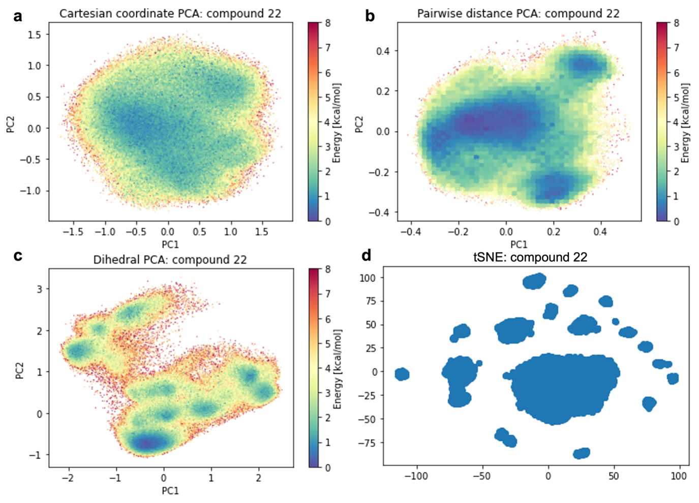
PCA performed with different inputs derived from the MD-trajectory. a) shows PCA with cartesian coordinates as input, b) shows pairwise N-O distances as input, c) shows reduced dihedral angles (phi, psi, omega) as input. d) shows the tSNE dimensionality reduction with dihedral angle inputs. See the interactive report to select parts of the PES and explore which structures this correspond to in the different representations.
The simulation trajectories contain the cartesian coordinates of all atoms. This high dimensional data (\(3*N_{atoms}\)) is too complicated to analyse by itself. To get an understanding of the potential energy landscape we applied dimensionality reduction. Fig. 3.8 shows the results of PCA for several different input features. The dPCA (Fig. 3.8 left) separated several distinct structures; other inputs (cartesian PCA, not shown here) were unable to separate the data equally well.
3.3.2. DBSCAN-Clustering
Note
Hover over a cluster to display additional information.
Fig. 3.9 Representative cluster structures plotted on top of the dihedral PCA. The x,y-axes show the first and second principal components, respectively.
Clustering was performed to identify representative conformers. In Fig. 3.9, we show the average cluster structures overlayed on the dihedral PCA based PES. While there are some redundant clusters and clusters that only capture a small fraction of the overall simulation frames, we found representative structures for most minima of the PES surface, independent of the PCA representation. To assess the structural variability of different representative cluster structures, we computed the RMSDs between all cluster structures in Fig. 3.10. The overall range of the observed RMSDs provides an estimate of the flexibility of the compound. The backbone RMSD between different clusters are maximum of 2.0 Å, indicating a moderately flexible compound.
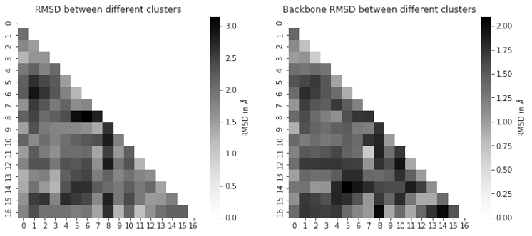
Fig. 3.10 RMSD between different clusters. The RMSD is given in Å. The x,y-axes both show the cluster numbers. The upper triangular combinations were omitted.
3.3.3. Computing NOEs and Comparison to Experimental NOEs
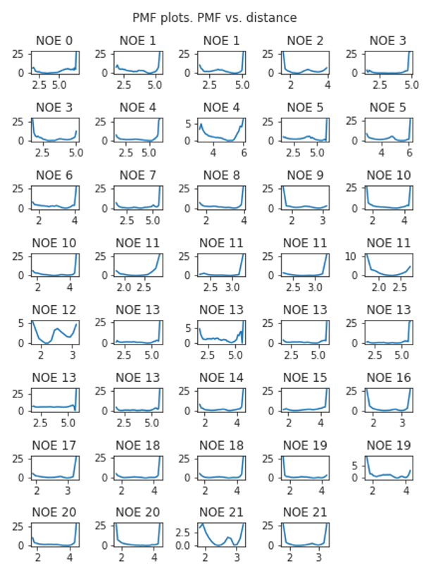
Fig. 3.11 Reweighted atom pair distances corresponding to NOEs. The x-axis shows the interatom distance in Å, the y-axis is the associated energy in kcal/mol.
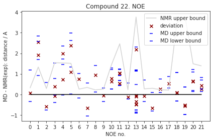
Fig. 3.12 Reweighted NOEs. This figure shows the difference between experimental NOE values and the average simulation values (red x, deviation). Also, we show upper and lower errors of the computed NOE values (MD upper bound, MD lower bound). These are also relative to the experimental NOE value and are computed as a population weighted RMSD analogues to Kamenik et al.[25]
As described previously, the NOEs distances were derived via reweighting and subsequent weighted \(r^{-6}\) Boltzmann averaging. The individual PMF plots of the reweighted distances are presented in Fig. 3.11. Fig. 3.12 shows the difference between the computed and the experimental NOEs. Generally, we observe good agreement of the computed NOEs to experiment, with only a few NOE-average values (#1, 6, 8) not within the experimental upper bounds (but the computed lower bounds are within the experimental upper bounds).
3.3.4. Statistics
In addition to visually inspecting different NOEs, we computed statistical metrics to evaluate how the simulated NOEs compare to the experimental reference. Overall, the RMSD is 0.45≤0.67≤0.90 Å, the mean signed error (MSE) is 0.00≤0.26≤0.52 Å, and the mean absolute error (MAE) is 0.34≤0.51≤0.70 Å.